Resistance thermometers Pt100 are precise temperature sensors widely used in a variety of industrial and scientific applications. Their principle is based on the variation of electrical resistance of a platinum wire depending on temperature. The ‘Pt’ in Pt100 stands for platinum, the material the wire is made of, and the ‘100’ indicates that the resistance at 0°C is exactly 100 ohms.
Pt100 resistance thermometers offer a wide temperature range from -200°C to +850°C and are characterized by their high accuracy. Their resistance-temperature curve is nearly linear, which facilitates calibration and interpretation of measured values.
These sensors change their electrical resistance proportionally to temperature changes. The temperature coefficient is approximately 0.385 ohm/°C at 0°C. Pt100 sensors typically have two, three, or four connections. Accordingly, they can be used in various circuit configurations, including 2-wire, 3-wire, and 4-wire circuits.
To ensure accurate measurements, Pt100 resistance thermometers must be protected from external influences such as moisture and mechanical stress. This is often achieved by using protective tubes. Additionally, they should be regularly calibrated, either in specialized laboratories or using reference thermometers.
Pt100 sensors are used in numerous applications, including the food industry, laboratories, air conditioning technology, the automotive industry, and chemical process engineering.
Table of Contents
How do resistance thermometers work?
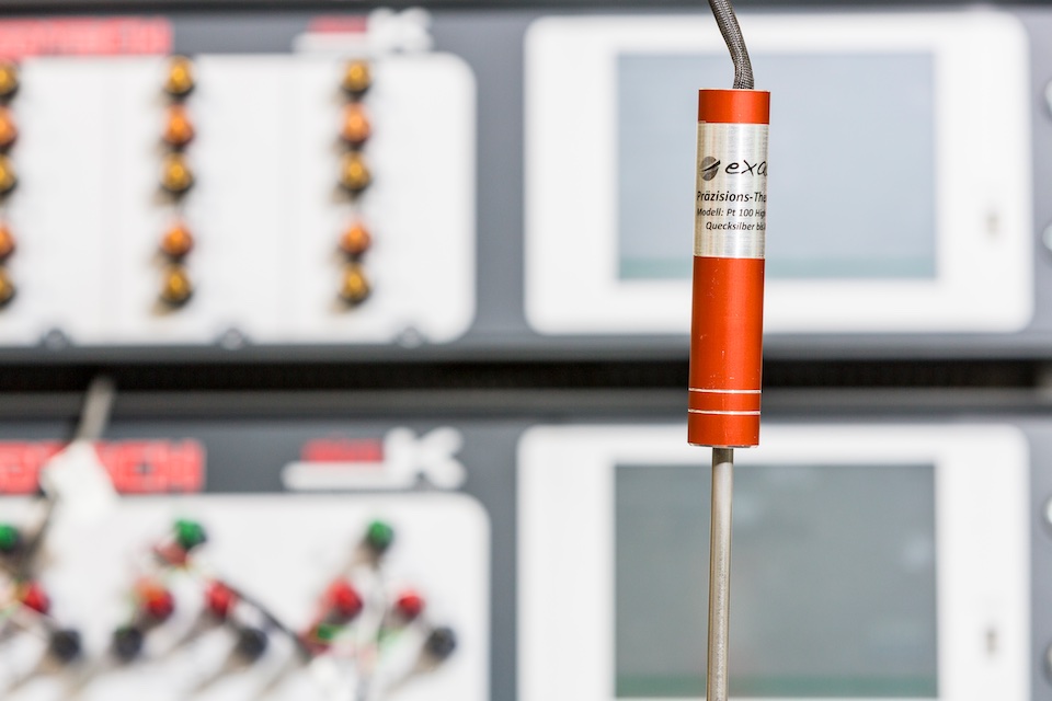
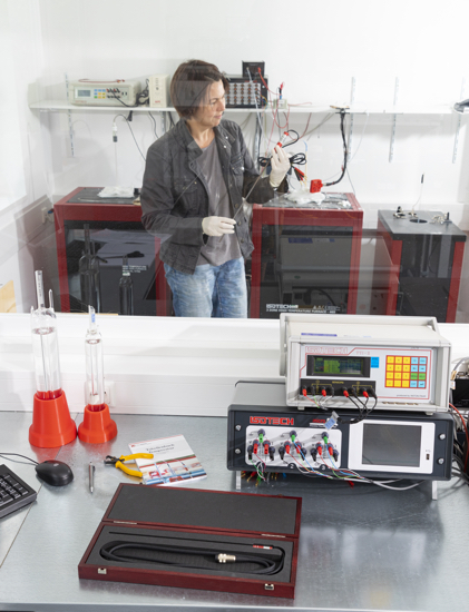
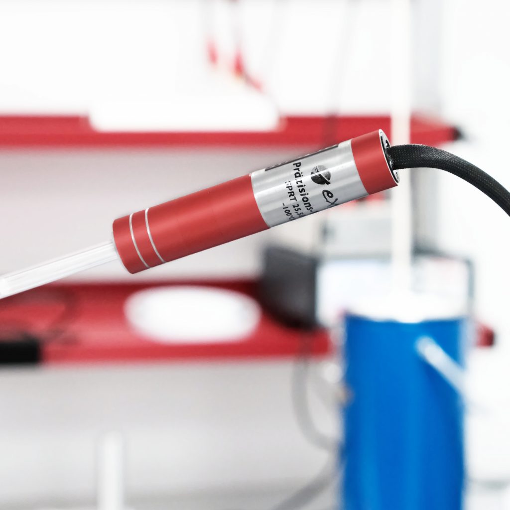
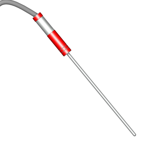
Resistance thermometers are frequently used for precise temperature measurements. The usual temperature range is between about -50 °C and 600 °C, although special applications exist where resistance thermometers are used from -200 °C to over 1000 °C. The depicted Pt100 resistance thermometer is from the calibration laboratory of Klasmeier.
The measuring principle of these thermometers is based on measuring the electrical resistance of measuring resistors, for which Ohm’s law is fundamental:
U = R ⋅ I = Constant
where:
U = Voltage,
R = Resistance,
I = Current
In school lessons, Ohm’s law is often represented as a triangle that illustrates the relationship between current, voltage, and resistance.
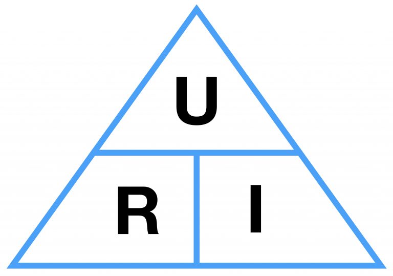
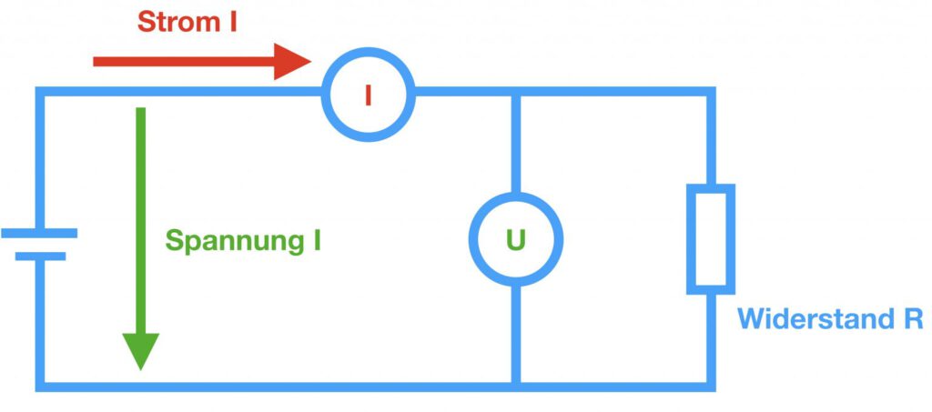
When two of these quantities are known, the third can be calculated. In the circuit diagram, Ohm’s law is represented as shown in the following graphic.
The relationships of resistance measurement and thus of resistance thermometers can also be graphically represented in a diagram.
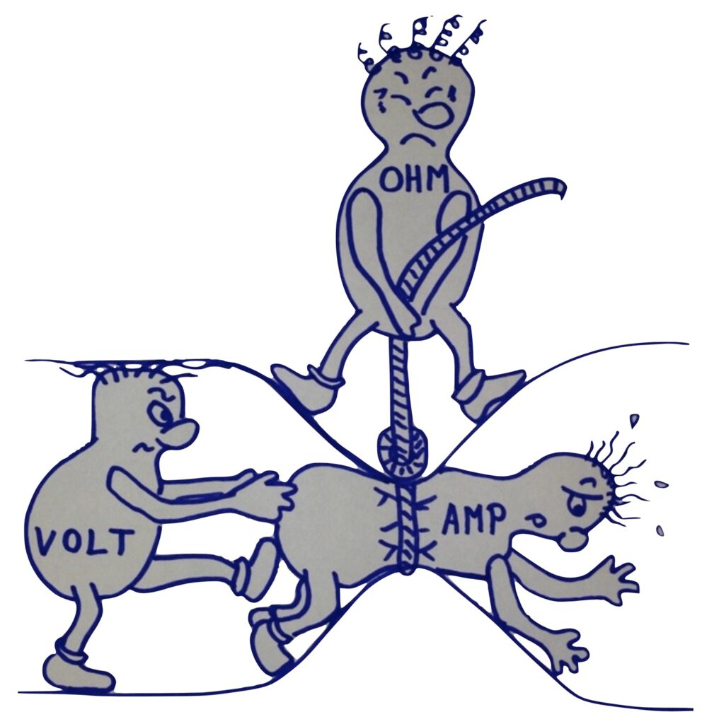
Here, the ‘VOLT-man’ (U – voltage) is pushed through a pipe by the ‘AMP-man’ (I – current), while the ‘OHM-man’ (R – resistance) tries to prevent this by narrowing the pipe. The success of the ‘OHM-man’ is temperature-dependent: The warmer it is, the harder it becomes for the ‘VOLT-man’ to move the ‘AMP-man’. Since this temperature-dependent effect is reproducible, the principle of electrical resistance measurement can be used for temperature measurement. A measured resistance R in ohms is converted into a temperature T in °C or K using a known relationship.
In principle, any electrical conductor that obeys Ohm’s law can be used as a thermometer. The specific resistance is the physical constant that describes this property. An overview shows the different specific resistances of materials at 20 °C.
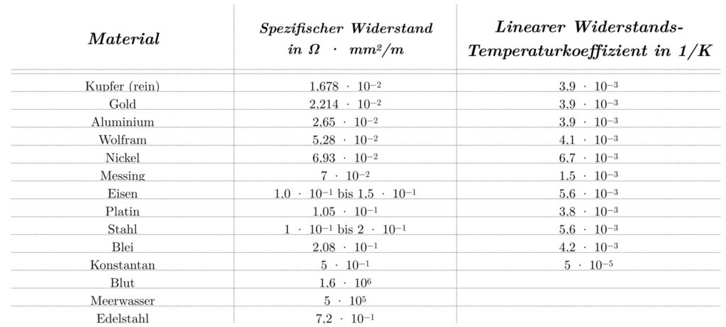
Although all mentioned materials can fundamentally be used for temperature measurement, there are certain selection criteria for choosing materials for thermometers. The material should have a high specific resistance and be generally suitable. For example, human blood has an excellent specific resistance of 1.6×10⁶ Ω⋅mm2/m, but it is not suitable for industrial production of thermometers. Metals are more suitable for this purpose.
In addition to the specific resistance, the linear resistance-temperature coefficient is also important. This describes the change in resistance of a material per degree Celsius and is given in 1/K. It can also be referred to as sensitivity. To minimize the requirements for measurement technology, this coefficient should be as large as possible. Therefore, the best compromise between cost, general suitability of the material, specific resistance, and resistance-temperature coefficient must be found.
Nickel and platinum have proven to be suitable materials. Initially, nickel measuring resistors, such as Ni100, were considered favorites as they showed higher sensitivity than platinum measuring resistors. However, they showed higher limit deviations and a limited temperature range. The standard for nickel thermometers, DIN 43760, was withdrawn in the 1990s. Since then, nickel measuring resistors have mainly been used in special technical applications.
Over time, platinum measuring resistors, such as Pt100, have become established. They are widely used in industrial measurement technology and today represent the standard for electrical temperature measurement with resistance thermometers.
The Pt100 characteristic curve for resistance thermometers simply explained
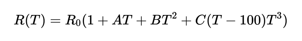
Platinum sensors have established themselves as resistance thermometers. The relationship between temperature and resistance in platinum thermometers is not proportional, but is described by a higher-order polynomial:

Here, the symbols mean:
R(T) = Resistance of the thermometer
R0 = Resistance of the thermometer at 0 °C
A, B, C, … = Individual parameters of the thermometer or standard
T = Temperature
In eigener Sache
Calibration of resistance thermometers
The company Klasmeier offers accredited calibrations according to DIN EN ISO/IEC 17025 (DAkkS) for resistance thermometers (e.g., Pt100, Pt25). The calibration is performed at temperature fixed points or using the comparison method, based on the DKD-R 5-1 guideline. The calibration range extends from -196 °C to 962 °C, and measurement uncertainties down to the millikelvin range are achieved.
Callendar-Van Dusen Equation
The Callendar-Van Dusen equation is a formula used to describe this relationship between temperature and electrical resistance of a platinum resistance temperature sensor.
The Callendar-Van-Dusen equation is also abbreviated as “CVD” and has been in use since the 1920s. The characteristic curve is standardized in DIN EN 60751, which describes industrial platinum resistance thermometers and platinum temperature sensors. It was first published in the 1990s and is still valid in its latest revision as DIN EN 60751:2009-05.
The Callendar-Van-Dusen equation itself can be formulated in two parts, for temperatures above and below 0 °C:
For temperatures T > 0 °C:

For temperatures T 0 °C:
Where:
- R(T) is the resistance at temperature (T)
- R0 is the resistance at 0 °C
- A, B, and C are coefficients that depend on the platinum resistance thermometer
In DIN EN 60751:2009-05, the coefficients for the Callendar-Van-Dusen equation are standardized:
A=3.9083×10 −3 °C-1
B=−5.775×10 −7 °C-2
C=−4.183×10 −12 °C-4
However, it is also possible to calibrate individual thermometers and calculate individual coefficients. This has the advantage that the thermometer no longer needs to be assessed based on the limit deviations of the standard, but can be individually adjusted to its own characteristic curve.
The Callendar-Van Dusen equation enables very precise temperature measurements by inserting the measured resistance of the thermometer into the Callendar-Van Dusen equation and calculating the temperature.
The following graph shows the two temperature ranges of the Callendar-Van Dusen equation. The temperature range from -200 °C to 0 °C is shown in blue, and the temperature range from 0 °C to 850 °C is shown in red.

The nominal resistance R0 of resistance thermometers
To better classify the measuring resistors, the so-called nominal resistance R0 was introduced in the DIN EN 60751 standard. This describes the electrical resistance of the temperature sensor at 0 °C. For example, a Pt100 temperature sensor has a resistance of 100 ohms at 0 °C. The following nominal resistances are listed in the standard:
- Pt 10 = 10 ohms at 0 °C
- Pt 100 = 100 ohms at 0 °C
- Pt 500 = 500 ohms at 0 °C
- Pt 1,000 = 1,000 ohms at 0 °C
Deviating nominal resistances such as Pt 25, Pt 2.5 or Pt 0.25 are used in precision thermometers and often meet the requirements of the ITS-90. These are then referred to as SPRT or standard thermometers. In laboratory applications, Pt 25 thermometers are often preferred as they offer a good compromise between stability, sensitivity, and self-heating.
Temperature coefficient in resistance thermometers
The difference between standardized thermometers and standard thermometers according to ITS-90 is evident in the so-called temperature coefficient, which is defined in the standard by a resistance measurement at 0 °C and 100 °C:
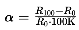
Here, the symbols mean:
alpha = increase of the thermometer in 1/K
R100 = resistance at 100 °C in ohms
R0 = resistance at 0 °C in ohms
The alpha value of industrial temperature sensors according to the standard is 3.85 10^-3/K, while the alpha value for standard thermometers according to ITS-90 is 3.92875 10^-3/K. This value corresponds to the sensitivity of spectrally pure platinum in this temperature range.
Sensitivity in resistance thermometers
The sensitivity of a resistance thermometer describes how strongly the resistance of the sensor changes in relation to a temperature change. It is a measure of how accurately the sensor responds to temperature changes. For a Pt100, the resistance changes by about 0.385 ohms for each degree Celsius change in temperature. This rate of change, known as the temperature coefficient, is a direct measure of the sensor’s sensitivity. Sensitivity is crucial for the accuracy and resolution of the sensor. A sensor with higher sensitivity can detect smaller temperature changes and allows for more accurate temperature measurements. This is particularly important in applications where precise temperature control is required, such as in laboratories or in process control in industry.
However, it should also be noted that temperature sensors with high sensitivity often have high self-heating and are less stable over long periods. Therefore, the ratio between nominal value and sensitivity of a temperature sensor must be chosen very carefully.
To achieve a defined nominal resistance, the length or diameter of the platinum wire in the measuring resistor is adjusted. This not only changes the resistance but also the sensitivity of the sensors to approximately:
- Pt 10 = 0.04 ohms / K
- Pt 100 = 0.4 ohms / K
- Pt 500 = 2 ohms / K
- Pt 1,000 = 4 ohms / K
In eigener Sache
eXacal Precision Thermometers
The eXacal precision thermometers from Klasmeier are designed for accurate temperature measurements and calibrations in a wide temperature range from -200 °C to 1200 °C. Available as resistance thermometers and noble metal thermocouples, they offer robust alternatives to ITS-90 standard thermometers. They are suitable for both industrial applications and laboratory calibrations and are hand-manufactured in the company’s own production facility.
Connection technologies of resistance thermometers
Resistance thermometers can be connected to measuring devices, data loggers, or measuring bridges, and there are various techniques for this.
- Two-wire technique
- Three-wire technique
- Four-wire technique
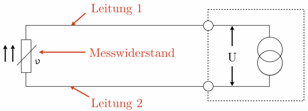
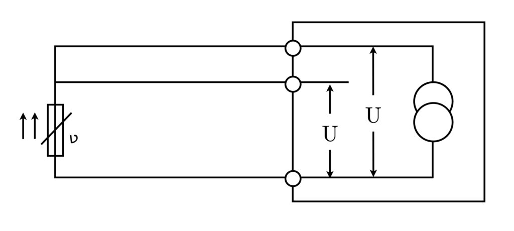
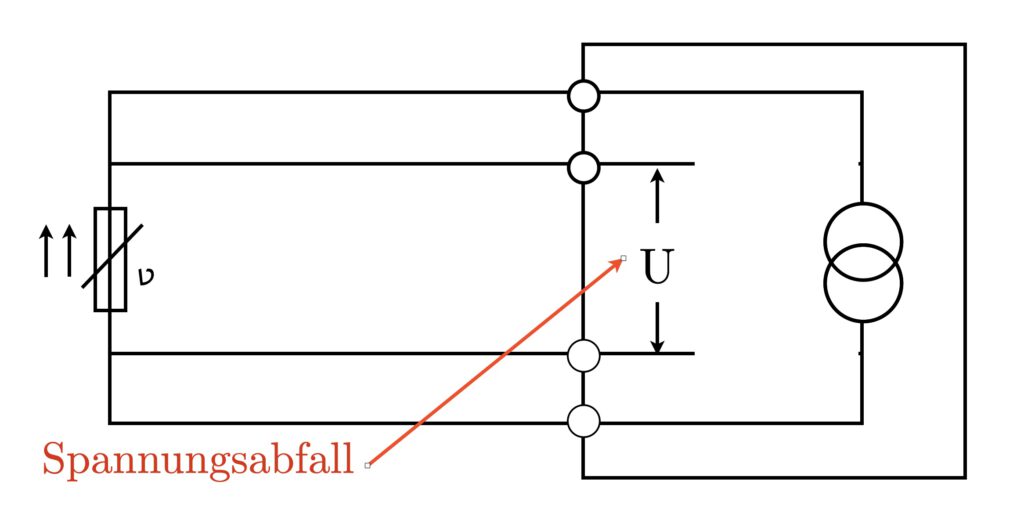
Two-wire technique
The two-wire technique demonstrates how to connect a temperature sensor to a measuring device, as shown in the image. It’s important to consider the resistance of the connecting cables, as they are connected in series with the measuring resistance.
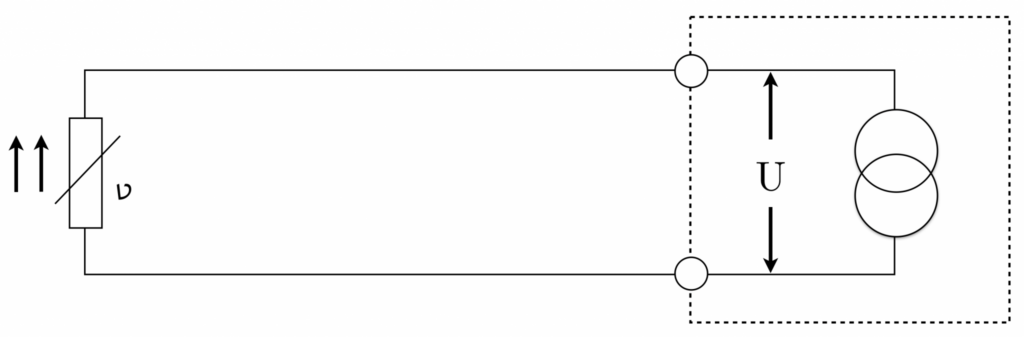
The resulting measurement is the sum of the resistance of wire 1, the measuring resistance (the actual temperature sensor), and wire 2, leading to an increased measurement. Therefore, correction of the measurement result is essential to eliminate measurement errors.
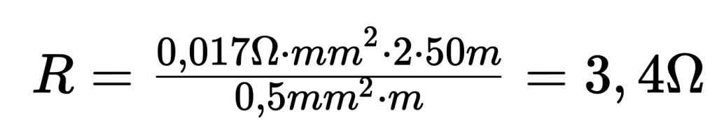
An exemplary calculation demonstrates the extent of measurement deviation under specific application conditions. Assume a temperature sensor is connected using a copper wire under the following specified conditions:
- Specific resistance of the copper wire at room temperature: 0.017
- Cross-section of the wire: 0.5 mm^2
- Length of the wire: approx. 50 m
The measurement deviation due to the connecting wire can be determined using the equation
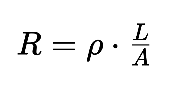
where:
- R represents the conductor resistance,
- ρ represents the specific resistance,
- L represents the conductor length, and
- A represents the cross-sectional area.
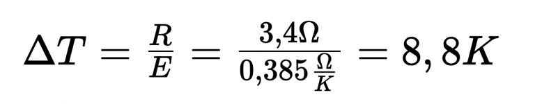
In this context, a conductor resistance of 3.4 Ohms results:
Considering a sensitivity (E) of a PT 100 temperature sensor of approx. 0.385 Ohm / K, this results in a measurement deviation of 8.8 K.
The wire length of approx. 50 m must be considered twice, for both the “outward” (wire 1) and “return” (wire 2) paths.
Historically, it was quite conventional to connect thermometers in production facilities using the two-wire technique. Before the era of digital technology, which simplifies the correction of systematic errors, correction tables were used to achieve accurate measurements.
An example illustrates correction values for a 10 m long connecting wire depending on the wire cross-section.

For a connecting wire with a cross-section of 0.5 mm^2, the resistance in a 10 m long two-wire circuit is 0.6 Ohm. This implies that the measured values must be corrected by this factor. For a Pt100, this corresponds to about 1.6 °C.
The following graph shows the correction values for a Pt100 in relation to the cross-section of a 10 m long copper wire in the two-wire technique.

Three-wire technique
The three-wire technique represents an improvement over the two-wire technique, particularly in terms of minimizing measurement errors due to wire resistances. In this configuration, three wires are used, with two wires connected in parallel to the measuring resistance and a third wire used to compensate for the wire resistance.
The compensation of the wire resistance is achieved through the measuring bridge, which takes into account the resistance of the third wire and thus subtracts the total resistance of the connecting wires. This results in a more precise measurement of the actual measuring resistance, as the influences of the connecting wires are minimized.
Although the three-wire technique represents a significant improvement over the two-wire technique, it is still susceptible to errors due to temperature changes and different wire lengths, which can affect the compensation of the wire resistance.
Four-wire technique
The four-wire technique, also known as Kelvin four-wire measurement, represents a further optimization in the precision of resistance measurement, especially for applications where the highest accuracy is required. This technique uses two additional wires to supply the measuring current and measure the voltage drop across the sensor, thereby eliminating the influence of wire resistance.
In this configuration, the measurement current flows through two of the wires (current wires), while the other two wires (voltage wires) are used to measure the voltage drop directly across the sensor. Since the measurement current does not flow through the voltage wires, the wire resistance of these wires is not included in the measurement, leading to higher measurement accuracy.
The four-wire technique is particularly advantageous for applications with low resistance values and long wire lengths, as it allows for precise measurement that is free from the influences of wire resistances.
In summary, the three- and four-wire techniques offer improved accuracy and reliability compared to the two-wire technique by minimizing or eliminating the influence of wire resistances. The choice of the appropriate technique depends on the specific requirements of the application, such as measurement accuracy, environmental conditions, and economic considerations.
In eigener Sache
Pt100 Model HS High-Temperature Precision Thermometer (0 °C to 850 °C)
The Pt100 High-Temperature Precision Thermometer from Klasmeier is suitable for precise measurements up to 850 °C. Equipped with a gas-tight ceramic protection and hand-crafted Pt100 measuring resistor, it offers only minor measurement uncertainties. Ideal for use as a calibration standard. Optionally available with accredited calibration according to DIN EN ISO/IEC 17025 (DAkkS).
Quellen
- Frank Bernhard: Handbuch der Technischen Temperaturmessung, 2. Auflage
- Thomas Klasmeier: Table Book “Temperature”, Edition 3
- Industrial platinum resistance thermometers and platinum temperature sensors (IEC 60751:2022)
- ISOTECH copper point thermometer No. 108462 up to almost 1100°C.
- Specific resistance
- DIN 43760
- Ohm’s law